A couple days ago, I decided to read OpenAI’s REPTILE paper. I decided to see how the algorithm worked in practice by implementing it for the simple case of a sine curve.
I wrote it in PyTorch. John already put up a gist in PyTorch, but this implementation is hopefully more idiomatic.
Correctly implementing it only took 90 minutes. Learning how to use Matplotlib well enough to confirm it was working took 2 days.
Typical.
The (Toy) Problem
Given a random sine curve, fit a neural network to it with few gradient steps.
You are allowed to first train on other instances of the problem, AKA random sine curves. So you want to learn how to learn a sine curve. Hence the meta in meta-learning.
We take a single minibatch and use that as training data for the true curve we’re trying to fit.
A Solution
Pick a set of starting weights, called meta_weights in my code and
\(\phi\) in the paper. (If you write a paper, you should use \(\theta\)
instead of \(\phi\) since that’s already standard and saves readers some
mental effort.)
Sample a random sine curve with amplitude \(a\) and phase \(b\) at points \((x, y)_{1:n}\) to get training data. Perform SGD for an arbitrary number of steps on a model parametrized by \(\phi\) to get a new set of weights, \(W\).
You can repeat the step above to get a minibatch of weights, \(W_{1:n}\). Then replace \(\phi\) with a weighted sum of \(\phi\) and the \(\theta_i\).
Assuming the minibatch size is 1, so we only have a single weight vector \(W\), the equation is:
\[\phi \gets (1 - \varepsilon) \phi + \varepsilon(W - \phi)\]You’re essentially finding a (weighted) center point between the weight vectors.
Hopefully, that weighted average will be a good set of parameters for solving the problem.
In the paper, they write it as \(\phi \gets \phi + \varepsilon(W - \phi)\), but I’ve always thought that’s a less clear way of writing what’s meant to be a convex combination.
That’s it. The algorithm is that simple. (They call it “remarkably simple” twice in the paper, but I think the code speaks for itself.)
On a more positive note, I’m glad the authors have a sense of humor. Check out Section 2 for what I mean.
Implementing a Solution
In a previous post, I talk about the relationship between weights and architectures.
In this problem, it’s more useful to focus on the weights rather than the architecture because the architecture is fixed across each model but the weights aren’t.
By overloading the state_dict of PyTorch (see ParamDict in
utils.py), we can perform arithmetic on weights directly and cleanly
implement our model.
The actual REPTILE function only takes 2 lines of code implemented
this way.
Performance
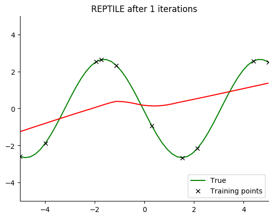
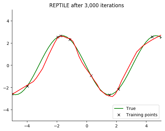
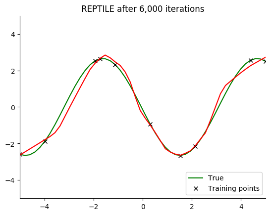
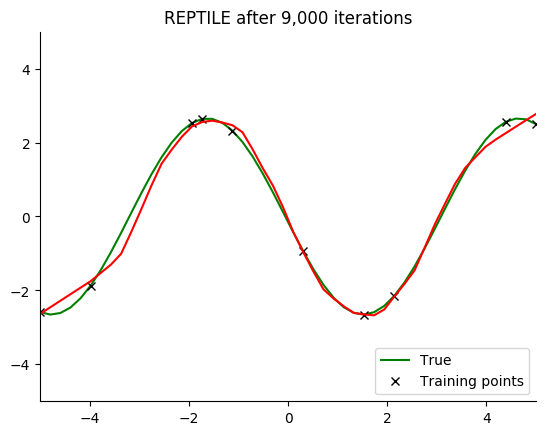
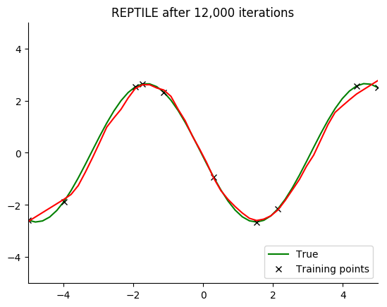
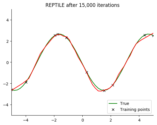
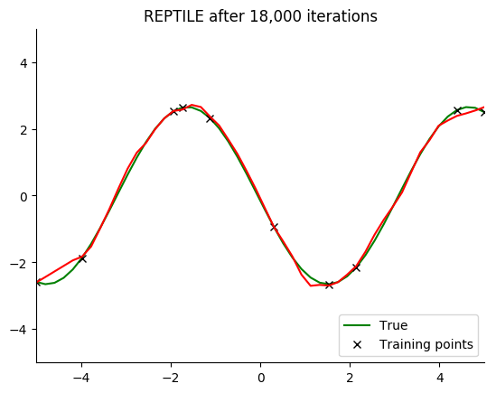
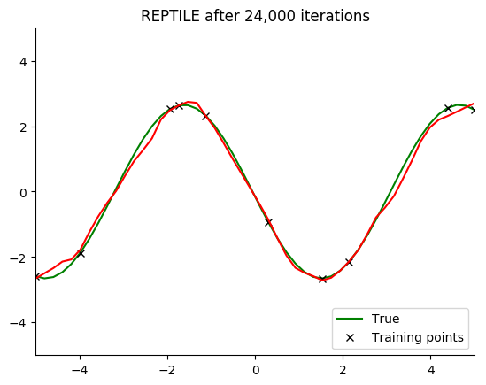
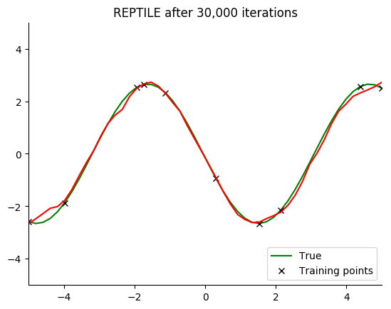
See for yourself. The green curve is the true sine wave we want to learn, and the red curve is the approximation after 8 steps of gradient descent from the current iteration of meta-training.
The black x are the points we train on for 8 steps.
Turns out that it works. You can even get a decent fit with just 2 gradient steps, but it isn’t reliable.
If you train on all the data rather than a single minibatch, 1 gradient step is enough.


Takeaways
I knew that the loss function isn’t always a perfect measure of what you actually want. But I didn’t really know it, since that knowledge was never as visceral as now.
This experiment made me truly appreciate the importance of hyperparameter tuning and plotting your work to ensure things are going as planned.
I learned the core abstractions of Matplotlib, and therefore how to actually use it. Now their documentation is useful to me. More to follow about that.